We examine the developments in trade patterns between the former Soviet republics in the years following the initial breakup shock. After a huge fall following the Soviet breakup of the early 1990s, Commonwealth of Independent States (CIS) trade with Russia began improving, and there have been recent formal efforts at Eurasian Economic Integration. This might be taken, a priori, as contrary to the hypothesis of gradual decline in Head, Mayer and Ries (HMR in J Int Econ 81(1):1–14, 2010)—or perhaps as evidence of the power of restored trade agreements, such as the incipient Eurasian Economic Union. We decompose the region’s trade into theory-consistent ‘gravity’ components, in order to analyze dynamic changes in the components since the Soviet era. Despite the sharp falls after 1991, trade in 1995 still shows strong ties, consistent with high dyadic (country pair) components linked to trade specialization. By contrast, in the second decade, the ties (dyads) began to weaken significantly and calibrated trade costs tend to rise, despite attempts at renewed integration. Rather, the sharp improvement in trade volumes was mainly due to the sharp recoveries in GDP levels for both Russia and many of the Central Asian Countries, associated with improvements in the global economy and economic ties with the World (especially with EU and China). We would therefore conclude that the recovery in trade between Russia and Central Asia reflects monadic factors (i.e., the regional economic recovery) and does not contradict the HMR (2010) hypothesis. Nevertheless, further, dynamic analysis shows that there are strong long-run ties within the CIS and Russia, which are not declining, and that sticky post-colonial adjustment does not appear set to eliminate the current bias of trade between these republics.
Avoid common mistakes on your manuscript.
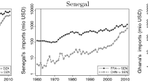
When an Empire breaks up, its legacy does not disappear overnight. In the last century, over 200 countries gained independence from their colonizers—especially after World War II. For example, when Algeria gained its independence in 1962, trade with its former colonial master (France) was around 80% of its total and after 30 years this fell to 6%. Similar patterns were observed throughout the other similar post-colonial relations. This is because colonialism diverts trade away from ‘natural’ trading partners to colonies/colonizers, but after independence, a former colony (as well as colonizer) will begin to build new economic linkages with countries outside its former colonial relationships. As a result, a post-colonial country like Algeria reduces its economic relations with the metropole (ex-colonizer) in favor of more ‘optimal’ trade partners and, consequently, the colony’s trade gradually begins to decline with its ex-colonizer. Nevertheless, the reorientation can be slow or sudden, depending partly upon the nature of the colonial breakup. Gravity analysis of trade patterns shows that trade between the former colonizer and colonies typically remains raised for decades after independence: for example, in 2004, France continued to account for 24% of Cote d’Ivoire’s exports. Trade with former colonial siblings also retains importance: for example, Ghana’s principal export destination is South Africa. These factors decline over time: sometimes rapidly, if independence leads to a nationalist backlash against the former colonist, but more typically, gradually.
In this context, we wish to explore a recent post-colonial experience—namely of the post-Soviet republics, and particularly those who re-joined to the Commonwealth of Independent States (CIS) and its associates, which we term ‘CIS+’. Table 1 in the next subsection provides a listing of countries in our study and their memberships of various groupings in the Soviet and post-Soviet eras. Note that we are using the term ‘CIS+’ because we are including Ukraine, in particular, which left the CIS recently, as well as Turkmenistan, which is not formally a member. Footnote 1 Prior to 1991–92, these were all bound together in a tightly integrated system, which was de facto dominated by (Soviet-) Russia, which we can perhaps view as ‘Big Brother’ of the post-Soviet republics. Russia remains by far the largest and most powerful member of the CIS+ club. Consequently, we choose to divide the CIS+ group into two: we term Russia the ‘metropole’ and all other ‘CIS+’ republics as ‘siblings’ to each other as they belong to the same former colonial group. We argue this is a valid distinction due to the dominance of Russia within the former Soviet Union (which did, after all, originate in the pre-1917 Russian Empire), and we use this division of the CIS+ into metropole and CIS+ siblings—‘SIB’—in much of our analysis below.
Soviet-era integration was very tight, especially given the lack of freedom to trade outside the Union of Soviet Socialist Republics (USSR). By contrast, pursuit of standardization and scale economies within the USSR led to integration of enterprises and distribution systems, under the control of Moscow-based ministries, the direction of transport infrastructure, strict control over external trade (semi-autarky for the USSR) and the spread of Russian-speakers as a diaspora across the republics, all of which integrated the republics tightly. In the post-Soviet period, and particularly since the economic stabilization after 2000, Russia has continued to seek close hegemonic ties, particularly with the relatively isolated and slower-reforming autocracies of Central Asia Footnote 2 in the form of a revival of a fledgling Eurasian Economic Union—formed by treaty in 2014, successor of the Eurasian Custom Union launched in 2011, whose current membership is Russia, Belarus, Kazakhstan, Armenia and Kyrgyzstan—as a more authoritarian rival to the European Union.
There are obvious limitations to data comparisons between the Soviet and post-Soviet eras. Nevertheless, the early breakup was very marked. Djankov and Freund (2002a, b) document that in 1990 all Soviet republics apart from Russia sent more than 80% of their exports to other Soviet republics, Footnote 3 while by 1996 most republics had undergone a significant realignment. This early breakup was clearly a major disruption, but for reasons of data continuity (pre-1991 trading prices were clearly distorted within the Soviet system, while after 1991 there were several years of hyperinflation), we prefer to focus our study on the period after this, from 1995. Looking at the former Soviet republics other than Russia, the share of trade with other ex-Soviet republics in this early breakup period was quite variable, with the Baltic States, whose breakup with the Soviet Union was hostile, among those seeing the sharpest falls, but also Tajikistan, Armenia, Ukraine and Azerbaijan. Moldova and Belarus, perhaps for geo-political but also economic reasons, continued their alignment with the other former Soviet republics.
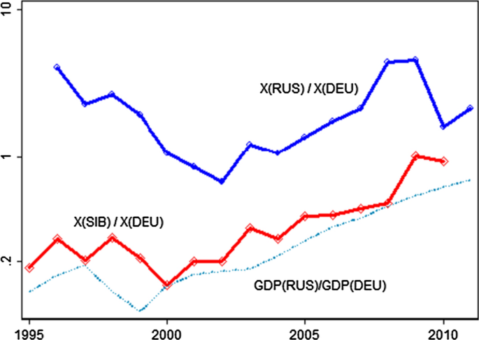
Our study focuses on the period subsequent to this. We acknowledge difficulties in deriving consistent data between the pre-1995 and post-1995 periods and focus on the latter. Most notably, during the post-1995 period, unlike the earlier period, trade started recovering sharply between former Soviet republics. For example, trade between the Central Asian former Soviet republics and Russia (the metropole), during the 1995–2014 period increased almost 11-fold from its post-Soviet nadir (from 2.1 to 23 billion U.S. dollars) and ex-Soviet republics’ shares in each other’s total bilateral trade actually increased. Footnote 4 The more Western republics have perhaps not moved as sharply back toward Russia—indeed, the Baltic States, Georgia, Moldova and, latterly, Ukraine, have begun orienting toward Europe—but the resumption of former Soviet trade ties is still apparent. This compares to the steadier decline in post-colonial ties indicated by Head, Mayer and Ries’ (HMR 2010) classic study, which examined the effect of independence on post-colonial trade of over 220 countries (including post-Soviets) between 1948 and 2006. Their work suggests that typically trade between a colony and its metropole (colonizer) erodes by 65% after 40 years passes since independence of the colony. Hence our paper starts by analyzing whether the sharp recovery in trade volumes between ex-Soviet countries since 1995 reflects a return to old ties, perhaps driven by policies (such as the various Free Trade Agreements, leading toward the institution of the recent Eurasian Economic Union), or whether the primary driver of recovery is simply the recovery of GDP, given stabilization and a recovery of oil prices after 1998. We review this below, although a first answer is that it is more of the second (recovery of output) than the first.
We do, however, investigate these issues more thoroughly in the rest of the paper. In particular, we develop and modify the gravity analysis of post-colonial ties developed by HMR (2010), to analyze post-Soviet relationships. In doing this, we find considerable heterogeneity between the post-Soviet republics. In this paper, we aim to strike a balance between acknowledging this heterogeneity, on the one hand, and seeking evidence of common trends, on the lines of other studies of post-colonial trade, on the other. We particularly favor the idea that ‘clubs’ of countries closer to Russia and further from it (politically and economically, rather than geographically) may help us understand the developments in the region.
In the rest of this section, we analyze the stylized facts of trade flows between the former Soviet republics. In Sect. 2, we discuss a basic gravity framework, following from HMR (2010), while in Sect. 3 we then start interpreting this in terms of potential factors which might influence post-colonial persistence in the former Soviet case. Sections 4 and 5 outline the data and discuss results, while Sect. 6 concludes.
The Soviet Union (USSR) was formally dissolved on December 26, 1991, ending a 70-year experiment in centrally planned integration between and within the republics. Table 1 lists all the countries in our study—these include 12 out of the 15 former members of the USSR. Footnote 5 The breakup was with varying degrees of hostility: in the first instance (de facto prior to the formal Soviet breakup), the three Baltic States (which had been occupied by Stalin after the Second World War) broke more or less completely with Russia (Rajasalu 1995), leading to the immediate imposition of sizeable trade barriers. These states never returned to any post-Soviet club, and eventually joined the European Union. Other states formed the relatively loose Commonwealth of Independent States (CIS), as listed in Table 1. This failed to prevent some conflicts between states, notably with the ‘metropole’ of the former Soviet Union (Russia), and eventually Georgia and recently Ukraine left the CIS.
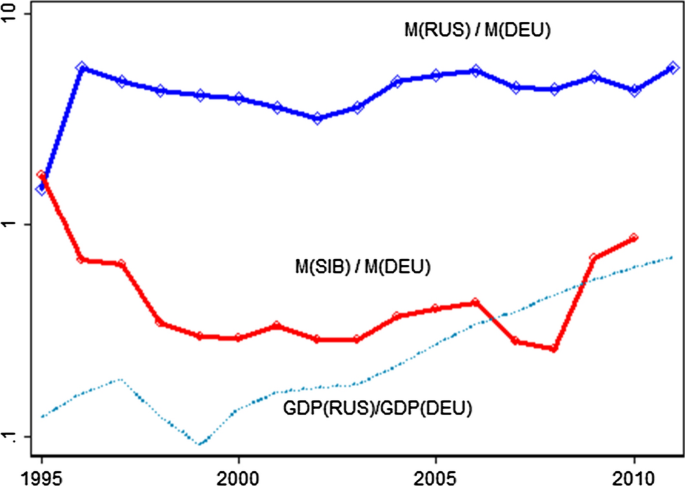
Separately, we construct the ratios for incoming trade flows in Fig. 2. The first line (the blue line) is CIS+ siblings’ (‘SIB’) imports (M) from Russia (RUS) divided by their imports from Germany (DEU), i.e., ( \(M_/M_\) ) and the second line (the red line) is CIS+ siblings’ imports (M) from the other siblings (SIB) divided by their imports from Germany (DEU), i.e., ( \(M_/M_\) ). Unlike Fig. 1 for exports, Fig. 2 shows that the average import from Russia compared to imports from Germany remains remarkably flat, after an initial uplift in 1996. The import ratio for siblings’ trade almost mirrors the former import ratio, especially in the first part, showing a sudden decline in 1996, then flat until 2007, with a ‘U-shaped’ dip, most likely caused by the financial crisis of 2008, followed by a renewed increase.
One question is whether, in fact, we are looking at post-colonial trade persistence which contradicts the HMR (2010) general findings. Footnote 7 To obtain the trade ratios we use the same bilateral trade data set obtained from World Integrated Trade Solution (WITS). An important caveat here is that we cannot derive the ratios for the initial (1991–94) trade collapse between the regions, due to a lack of good data. Footnote 8 Note that this is not inconsistent with observations of the even sharper trade realignment of the Baltic States (Rajasalu 1995), though in those cases the fall was even more acute, due to trade sanctions in response to their decision to leave the Soviet Union and not to enter the CIS. Indeed, both the Russian and CIS+ economies endured huge trade and production hardships with the Soviet collapse and subsequent hyperinflation in 1991–95. In fact, the disruption of what had been integrated supply chains by managerial independence, the introduction of border controls and initial currency convertibility issues, is often cited as a major cause of the collapse of output across the former Soviet Union in this period (see, for example, Linn 2004).
In order to examine changes in the relative orientation of trade presented in Figs. 1 and 2, it is useful to look at trade ratios of each individual CIS+ sibling member with Russia. These are shown in the two parts of Fig. 5 in ‘Appendix.’ Most CIS+ countries share similar trade patterns to those shown in Figures 1 and 2; however, there is some heterogeneity. Some CIS+ countries (Kyrgyzstan, Uzbekistan and Tajikistan) had above average export ratios toward Russia, while the oil exporters such as Kazakhstan, Turkmenistan and Azerbaijan had reoriented their exports toward the rest of the World (non-USSR). Country-level import ratios suggest that only Uzbekistan and Kyrgyzstan (which are isolated from Europe) and Belarus (which clung faithfully to Soviet standards) were above average in terms of relative import share from Russia, while Ukraine and Moldova had joined Lithuania in shifting imports toward Germany.
Although it started as a purely empirical model, in recent decades, the gravity model has been given a sound theoretical grounding, associated with various trade models: in the case of the Armington model, Anderson and van Wincoop’s (AvW 2003) paper is seminal, while Bergstrand (1989) links gravity to Krugman’s ‘love of variety’ model. Deardorff (1998) produced a Heckscher–Ohlin derivation, while Eaton and Kortum (2002) adopted a Ricardian approach. More recent trade theory developments are incorporated by Chaney (2008), Helpman et al. (2008) and Head and Mayer (2014).
In this paper, we analyze post-Soviet trade flows between the countries which we term ‘CIS+’—especially between the metropole, Russia and the siblings—from the perspective of the structural gravity framework that explains trade flows in terms of ‘monadic’ (country-specific) and ‘dyadic’ (country-pair-specific) factors. This can be summarized by a standard panel gravity equation for trade between countries i and j in year t:
$$\beginIn this framework, \(x_\) is the trade flow from i to j at time t which is equal to \(g_\) , a ‘global’ factor (such as the value of global trade), which can usually be proxied with a series of year dummies; \(m_\) and \(n_\) are the ‘monadic’ (or country-specific) factors, comprise economic output (GDPs) and overall openness to trade (as measured in the form of ‘multilateral trade resistance’ by AvW (2003); and \(d_\) is a set of ‘dyadic’ factors , which refer to country-pair-specific factors, such as transport costs (related to distance), colonial and language ties and a common border, which are statistically and economically significant. Using a variety of methods, we analyze dynamic changes in the components over the period 1995–2011, differentiating between monadic (country-specific) and dyadic (country-pair-specific) factors.
Looking first at the role of monadic factors: in the first decade after Soviet breakup, these were weak, and explain much of the initial collapse. Economic disruption and the weakness of primary product prices (Russia, Azerbaijan and much of Central Asia all being dependent on primary product exports, while Ukraine was dependent upon pipeline rents, at least until after the Orange Revolution of 2004–05), meant that GDP in both Russia and the CIS+ siblings was well below Soviet levels. Indeed, once we correct for the overall effects of the initial fall in economic output, the dyadic pair-specific component (including Soviet built socioeconomic CIS+–Russia ties) in trade was still strong in the first decade of CIS+ independence, in the sense that Russian-sibling trade remained well above the distance-adjusted GDP ratio. However, in the second decade, our analysis shows that these dyadic ties were weakening significantly (in line with the HMR (2010) finding of eroding post-colonial trade relationships). Against, this, GDP in most of the CIS+ states began to improve fast after 2000, as economies were stabilized and as primary export prices recovered.
In analyzing the relationships between the CIS+ siblings and the metropole (Russia) but also relationship of the siblings with each other, we need to note that there is a good deal of heterogeneity in the post-colonial paths of these countries. In this paper, we aim to strike a balance between acknowledging this heterogeneity, on the one hand, and seeking evidence of common trends, on the lines of other studies of post-colonial trade, on the other hand. We particularly favor the idea that ‘clubs’ of countries closer to Russia and further from it (politically and economically, rather than geographically) may help us understand the developments in the region. Indeed, irrespective of which of the various theoretical foundations is chosen, all these studies broadly conform to the gravity model expressed in (1). Further to provide more insight into our regression results, we restate (1) using AvW’s (2003) Armington-based structural gravity form:
$$\beginwhere on the left side, \(y_\) is output in i, \(y_\) is expenditure in j, \(\tau _\) is the bilateral iceberg type trade cost and \(P_\) and \(P_\) are exporter and importer multilateral resistances (CES aggregate prices—see below) at time t.
The monadic components, \(m_\) and \(n_\) , are the sets of unique attributes that are only in the possession of i or j, respectively, at time t explaining the trade flow between the pair. The monadic component of any i comprises positive (GDP, \(y_\) ) and negative (local composite price index of ‘multilateral resistance,’ \(P_^\) ) attributes, and can be written as:
$$\beginTheoretically speaking, local output, \(y_\) , is equal to the sum of gross consumption \(c_\) of i’s produce across all countries j (including i) at a price ( \(p_\) ) at time t that differs from j’s domestic price level by the inclusion of a trade cost ( \(\tau _\) ):
$$\beginRegion j’s economic size at time t ( \(y_\) ) is calculated analogously. It is common practice in a gravity analysis to proxy economic size using the nominal GDP of the country, or by collecting bilateral trade flows by either i or j. Footnote 9
An important component of Eq. (3) is the multilateral resistance to trade (MRT) term, the central contribution of AvW (2003). The outward trade resistance of exporter region i at time t, \(P_\) , is price index that takes into account the weighted aggregate values of observable traded costs ( \(\underset\tau _\) ) and income share ( \(\underset\theta _^>\) , where \(\theta _=\frac
Here, \(\sigma\) is the CES elasticity of substitution between domestic and imported goods. The parameter should be larger than one, but exact values may change as preferences and trade opportunities change. Some studies try to estimate it (e.g., Chen and Novy 2012) or calibrate it (e.g., Balistreri and Hillberry 2008) but most studies introduce it exogenously by assigning a level to it. The inward trade resistance of region j at time t, \(P_\) , is derived in similar fashion just by replacing i and j in (6). Both inward and outward MRT terms are not directly observable, though gravity studies provide methods to construct them (see Anderson and Yotov 2010).
The global factor ( \(g_\) ) is the scale of the global economy, which plays a role of a scale parameter in the gravity equation, and it is equal to the sum of nominal incomes collected either by i (or j) at time t:
$$\beginIn the era of globalization and intense integration, a country builds more trade linkages with other countries (through liberal reforms, trade agreements or trade unions, etc.) and becomes a part of bigger economy (global or regional economy). This way a country whose economic size is \(y_\) forms a part of World economy size ( \(\undersety_\) ) and depending on the countries relative to World economic size and nature of networking, changes in (2) can affect the left-hand side of (1) either positively or negatively.
The dyadic component ( \(d_\) ) is a trade cost associated with physical and psychic distances (and quality) in each unique (specific) ijt set:
$$\beginwhere trade costs, \(\tau _=\underset\left( z_^\right) ^<\gamma _>\) , comprise the combined effect of a series of bilateral physical (geographic distances, transport mode, quality of transport infrastructure) and psychic (or non-physical) trade barriers (tariffs, quotas, language, etc., indexed m), and are assumed symmetric in both directions, and of ‘iceberg’ form (Samuelson 1952). The geographic distance between trading countries i and j commonly serves as a proxy for transport cost. Psychic distance is not directly observable, but can be proxied by a set of attributes (such as language barrier, adjacency and colonial history), which are commonly found to important in gravity-based studies. For instance, HMR (2010) used year dummies to capture the growing effect of independence on trade relations between a former colony and metropole. However, some dyadic barriers (such as tariffs) can change from year to year while other types of barriers (geographic distances) would be constant.
Because we are interested in the time-varying effect of independence on trade between a metropole (colonizer), colony and siblings (other colonies), in the Soviet Union context, apart from standard gravity analysis, it is sensible for us to adopt the so-called Tetrad method. HMR (2010) show that by taking a ratio of ratios of bilateral trade flows (i.e., a tetrad of the flows) in the following form we can obtain \(t_\) , a tetrad of the dyadic components:
$$\beginwhere x denotes bilateral trade flow and additional subscripts (k and l) stand for two particular reference countries. This is well explained in HMR (2010) study but essentially we can understand (9), if we replace x’s with gravity components on the r.h.s. of (1), the monadic and global constant components cancel out leaving \(\frac/d_>/d_>\) alone. Because \(d_=\tau _^\) , and given that \(\sigma\) is the same across all countries, then (9) is also a measure of trade costs (both observable and unobservable costs) relative to their level at two chosen reference countries (l, k):
$$\beginMore detailed discussion on this method is in HMR (2010).
In this paper, we are testing whether post-Soviet Russian-other CIS+ sibling ties broadly conform to the usual post-colonial pattern of gradual decline, led by rising relative trade costs between former colonizer and its colonies. However, no group of countries is identical to any other, and we therefore need to take careful account of other factors—monadic and dyadic—which might affect the dynamics of trade change, given the mass geography of the region.
We would like to start with some key concepts. Trade volumes react to changes both in trade costs and in economic activity. Studies of the erosion of post-colonial ties (such as HMR 2010) normalize for changes in economic activity by utilizing a gravity framework, which eliminates the effect of GDP changes. We need to bear in mind that the recovery in trade volumes between Russia and CIS+ siblings will, in part, be responding to the recovery in economic output of the two regions between 1998 and 2008, in turn reflecting a global commodities boom and a bounce-back from the initial disruption of the Soviet breakup.
We note that GDP growth, when it occurs in both the exporter and importer countries, has a compounded effect on bilateral trade volumes. For example, if we use the simpler format in Eq. (2), where the elasticity of trade volume with respect to both exporter and importer countries is set at 1, then if GDP of both halves (which is not a bad approximation of the post-Soviet collapse) then we might expect trade between the two countries to fall by 75%, while if exporter and importer GDPs subsequently double again, bilateral trade will quadruple. Footnote 10 Since gyrations of GDP in the post-Soviet era have been extreme, we would expect to have to correct for these large compounded effects, before we can actually start working out what is happening to post-colonial trade bias.
Remoteness and inaccessibility are also important factors in determining trading patterns, especially in the context of landlocked former-USSR countries and even some remote parts of Russia. Any factor which raises trade costs on one route will lower trade (negative dyadic factor), but at the same time raise the overall price level within the nation concerned (monadic factors offsetting the effects of raised trade costs with any one partner). This is worth bearing in mind in the section below, as we discuss dyadic factors.
It is worth noting that all of the CIS+ countries were colonized by Russia gradually well before the Russian Revolution. Footnote 11 The number of Russian colonists in Siberia rose to 2.7 million by 1850. The Caucasus was largely gained following the Crimean War. In Central Asia, Tashkent fell to the Russians in 1865. The Trans-Siberian Railway was built between 1891 and 1916, while the Russians had also built railways into their Central Asian territories before the First World War. With the railways came settlement: the 1897 Census shows ethnic Russians were already 12.8% of the population of Kazakhstan in 1900, with Russian farmers settling in Northern Kazakhstan in the 1890s. This rose to over 20% in 1926, and 40% in 1939, as Stalin’s forced movement of Soviet peoples took hold.
Hence, historically, we are looking at regions which began integrating with Russia in the last decade of the nineteenth century, but whose integration was accelerated by the Soviets. Consequently, colonial ties can be seen as predating the Soviets, but were strengthened during Soviet rule.
The CIS+ countries occupy a vast and mostly sparsely populated, landlocked area. In this regard, the most extreme cases are the Central Asian states, which are not only landlocked, but also bounded to the South and East by mountains and deserts. Limao and Venables (2001) estimate that overland transport costs of goods averaged $1.380/1000 km, almost 10 times higher than by sea ($190/1000 km), and Carrere and Grigoriou (2007) found an additional transport cost, freight cost is $500/1000 km. The easiest overland trade routes are north-westward into Russia, and Russian goods will face less competition from other countries, simply because the Central Asian states will face even higher transport costs to get the goods anywhere else. In AvW’s (2003) terminology, the multilateral resistance price is high in these countries, which means that trade with Russia will be greater than might otherwise be inferred from size and distance.
Raballand (2003) found that the trade of landlocked former Soviet countries, compared to coastal ones, fell by 80% during 1995–1999 period, so landlocked Central Asians, if they wanted to trade, had to negotiate with bordering coastal Russia, to access its sea transport channels (Carrere and Grigoriou 2007). Djankov and Freund’s (2002a, b) study, which focused on border effects on trade, estimated that (non-physical) trade barriers imposed by coastal Russia to landlocked Central Asia were very high compared to trade barriers imposed by coastal states to landlocked ones in the OECD area.
A key implication of this is that, even though Russian-Central Asian trade may have been inflated by excessive Soviet era integration (and trade barriers with the rest of the World), these countries, unlike many other former colonial groupings, can still be seen as natural trading partners, and hence we would expect a smaller long-run decline.
For other republics: Armenia is landlocked and has a relatively isolated mountain location, especially given its poor relations with its immediate neighbors (Turkey and Azerbaijan). Even for Azerbaijan, the political effects of conflicts in Georgia and Chechnya will have deterred trade.
In this regard, the more Westerly former Soviet republics had much easier contact, at least with Europe. The Baltic States, which joined the EU, not the CIS, have easy sea links to the West. Ukraine and Moldova also border the EU, as does Belarus, although in this latter case political isolationism is an important offsetting factor.
The former Soviet republics have dated transport connections, dominated by Soviet transport infrastructure connecting Russia and the CIS+ siblings. Most traded and transit goods of both regions rely on those railroads (for the Central Asian republics, for example, it is about 90%). The railroad net mostly covers western Russia and Kazakhstan. Carrere and Grigoriou (2007) argue that infrastructure and railroads built during the Soviet era are an important factor in determining with whom Central Asian republics will choose to trade (meaning with Russia and the CIS+ Siblings). Footnote 12 Footnote 13 Further West, Ukraine and Moldova, Belarus, Azerbaijan and Georgia have begun to benefit from EU neighborhood investments in transport and port infrastructure, particularly under the Eastern Partnership Transport Panel, established in 2011. Footnote 14 It is worth noting that the imposition of national borders can increase delays and hence worsen infrastructure: Djankov and Freund (2002b), found that between 1989 and 1996, train speeds increased by an average of 2% between Russian regions, but slowed by an average of 5–6% between Russian regions and other former Soviet republics.
There was considerable migration between what are now the CIS+ republics before and during Soviet times. For example, even now each 10th citizen of Russia is Central Asian (17.8 million) and each 10th Central Asian citizen is Russian (6.72 million) (Central Intelligence Agency 2018). The majority of this migration occurred during the Soviet era, and was permanent enough for at least one generation to be born in their new adopted homes (Table 2). These migrant diasporas create long-lasting social and cultural connections between the regions and have an important impact on the economic and political relationship between Russia and the Central Asian countries.
The results of four dynamic estimations are summarized in Table 7.